The computations and the software for data analysis should be trustworthy: they should do what they claim, and be seen to do so (Chambers 2008, 3).
The only way to write complex software that won’t fall on its face is to build it out of simple modules connected by well-defined interfaces, so that most problems are local and you can have some hope of fixing or optimizing a part without breaking the whole (Raymond 2003, ch. 1).
Introduction
Code for a data analysis should be accurate, transparent, and flexible. It should do what the report on the analysis say it does, and it should be written in a way that makes it easy to understand and modify. In software engineering, and in the design of systems more generally, one of the key ways of achieving accuracy, transparency, and flexibility is through modularity (Simon 2019). A modular system is built out of many small, self-contained units. Each of these units has a single purpose, has well-defined inputs and outputs, and has only limited knowledge about other units.
Ideas about modularity underlie much standard R advice about writing
code for data analysis. RStudio-style projects, for instance, are an
example of modular design (Wilson et al. 2017;
Wickham et al. 2023; ProjectTemplate contributors 2025). However,
many actual data analyses written in R are the opposite of modular. For
instance, the entire workflow is often contained in a single, huge
script that is responsible for everything from importing data to fitting
to creating plots. Even when code for an analysis is divided into
smaller scripts, these smaller scripts often have diffuse aims and
complex inputs and outputs. Heavy use of source() commands
mean that many scripts contribute objects to the current working
environment, and no script can be understood in isolation. Changes to
one part of a workflow have large, unexpected implications for other
parts of the workflow.
This article presents a strategy for making data analysis workflows more strictly modular. The basic unit in this strategy is a script. Each script is responsible for one small task, with inputs and outputs tightly controlled. Each script runs in its own environment, and data and intermediate outputs are passed around by reading from and writing to disk. Information about the project as a whole is held in a single orchestration file, which serves as an executable description of the analysis.
The article describes the main elements of the strategy, presents an example, and lists some costs and benefits. The final section gives some suggestions about implementation details.
A strategy for constructing a modular workflow
Use lots of small scripts
A data analysis workflow should be composed of many small scripts. Each of these small scripts should have a single well-defined task. In most cases, the task will be to turn some inputs into an output. The new output could itself be an input for other tasks, or it could a final product, such as a report. In either case, each script should be self-contained, in the sense that it can be interpreted and used on its own.
Some typical inputs and outputs in data analyses are:
| Input | Output |
|---|---|
| Raw data set | Cleaned data set |
| Two cleaned data sets | Single merged data set |
| Cleaned data set | CSV file for distribution |
| Cleaned data set | Values for plotting |
| Values for plotting | Plot |
| Cleaned data set | Fitted model object |
| Cleaned data set and fitted model object | Actual and predicted values |
| Actual and predicted values | Plot |
| Multiple fitted model objects | Scores for performance metrics |
| Scores for performance metrics | Values for table |
| Values for table | Table |
The one-task-one-script rule can lead to scripts that are very short. For instance, if the task is to merge two cleaned datasets, then the script might contain only a few lines of code.
Occasionally, a script does need to be long, because breaking the task into subtasks increases, rather than decreases, complexity. A long script should, however, be subjected to extra checking, and should include a comment explaining to future maintainers why the extra length was necessary.
Use Rscript or littler to run each script in a new session
Each script should run in a new, clean R session that ends when script has finished running. Any packages (aside from base R packages) that are required by a script should be loaded explicitly. Running each script in its own session implies that, when the script completes, all objects created during by the script that were not saved to disk disappear.
The best way to give each script its own session is to run the script from the command line, using an application such as Rscript or littler. For instance, the call
starts a new R session, runs the code in my-script.R,
and ends the session.
For an introduction to Rscript see here, and for an introduction to littler, see here.
Use command line arguments to define inputs and outputs
Rscript and littler both allow the user to supply command line arguments to the script being run. Values for these arguments are accessible inside the session. The command
for instance, makes the strings "my-data.csv",
"myoutput.rds", and "3" accessible inside the
session where my-script.R is run. Expressions of the form
--<name>=<object> can be used to assign names
to the strings. In the command above, for example, the strings
"my-data.csv" and "myoutput.rds" have no
names, and the string "3" has the name
n_digits.
Values for command line arguments can be retrieved within the session using base R function commandArgs(), followed by some manipulation and reformatting. For instance, values from the call above can be retrieved using
args <- commandArgs(trailingOnly = TRUE)
filename_input <- args[[1]]
filename_output <- args[[2]]
n_digits <- as.integer(strsplit(args[[3]], split = "=")[[1]][[2]])
As this example illustrates, using base R function
commandArgs() to parse command line arguments can be
fiddly. Packages argparse, docopt,
getopt, optparse, and R.utils all
implement high-level alternatives to base R commandArgs()
(Jonge et al. 2018; Davis 2023; Pav 2023; Davis
and Day 2020; Bengtsson 2023).
The command package is one further alternative, designed
specifically for data analysis workflows. Function
cmd_assign() in command automatically checks
and reformats arguments, and assigns values within the working
environment. For an introduction to command, see Quick
Start.
The ability to pass arguments to scripts essentially turns the
scripts into functions. If, for instance, we want to run the code in
my-script.R on my-other-data.csv, rather than
my-data.csv, then we use something like
If we want to process my_data.csv, but we want to use 5
digits rather than 3, then we use something like
Run everything from an orchestration file
An orchestration file controls a workflow. Running the orchestration file for an analysis should reproduce the entire analysis, from the ingesting of the raw data to the compilation of the final report.
Orchestration files are often written in R, and take the form
source("cleaned_data.R")
source("model.R")
source("performance.R")
quarto::quarto_render("report.qmd")
The script runs cleaned_data.R to create a cleaned
dataset, runs model.R to fit a model to this dataset, runs
performance.R to collect information on model performance,
and renders the report.qmd file to create the analysis
report.
Orchestration files consisting of a succession of
source() calls have major some disadvantages. Repeated use
of source() means that all code is run in the same
environment, breaking modularity. The lack of definitions of inputs or
outputs make the workflow harder to understand or control.
A better approach is to use a shell script, such as
Rscript cleaned_data.R raw_data.rds cleaned_data.rds

Rscript model.R cleaned_data.rds model.rds --n_iter=2000

Rscript performance.R model.rds performance.rds

quarto render report.qmd
An even better approach is to use a Makefile. A Makefile version of the shell script above is
.PHONY: all
all: report.html

cleaned_data.rds: cleaned_data.R raw_data.rds
        Rscript $^ $@

model.rds: model.R cleaned_data.rds
        Rscript $^ $@ --n_iter=2000

performance.rds: performance.R model.rds
        Rscript $^ $@

report.html: report.qmd performance.rds
        Rscript $<
The lines
at the top of the Makefile define the final output or outputs from the workflow. Lines such as
specify a Makefile rule. A rule contains a
- a target, in this case
cleaned_data.rds; -
prerequisites, in this case
cleaned_data.Randraw_data.rds; and - a recipe for creating the target from the prerequisites, in
this case
Rscript $^ $@.
The $^ and $@ in Rscript $^ $@
are “automatic variables”. When the Makefile runs, the phrase
Rscript $^ $@ expands to
Rscript cleaned_data.R raw_data.rds cleaned_data.rds.
The make application uses the Makefile to construct a
dependency graph for the inputs and outputs in the workflow. The
Makefile above yields the graph
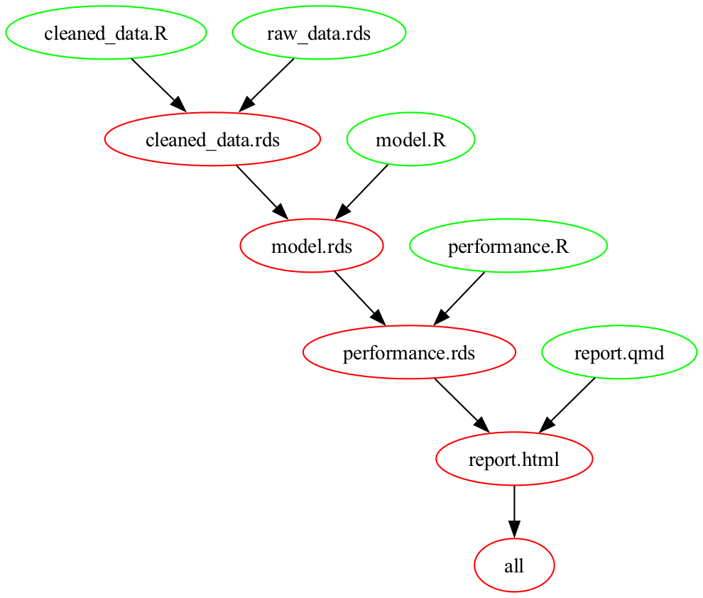
If make sees that a dependency is older than one of the
prerequisites, then it will recreate that dependency, and all
dependencies downstream of it. For instance, in the example above, if
make saw that performance.rds was older than
model.rds, then it would recreate
performance.rds and report.html. It would not,
however, create model.rds itself, or
cleaned_data.rds. For more on Makefiles, see, for instance,
Broman (2013), Baker (2020), Janssens
(2021), and The Turing Way Community
(2025).
Reports
Applications such as R Markdown (Xie et al. 2018) and Quarto (Posit Software, PBC 2025) allow authors to combine code and text within a single document. It is common to see authors put all the code for an analysis in an R Markdown or Quarto document. This can be effective with small analyses, such as the exploration of a new dataset. But it does not scale well. Analyses where all the code is contained in a single R Markdown or Quarto file suffer from all the usual pathologies of a large, complicated code file, along with the extra challenge of coping with markdown errors.
A more modular, scalable alternative is to do the analysis outside
the report, and to limit code within the report to snippets that read in
results and apply formatting. A plot, for instance, can be constructed
in its own script, and then read into the report using a command like
.
Unfortunately, R Markdown and Quarto do not currently allow users to supply command line arguments in the way that Rscript and littler do.
An example
We use a small example to illustrate the various components of the strategy described in this paper. The project folder for the example looks like this:
.
├── Makefile
├── data
│ └── raw_data.csv
├── out
│ ├── cleaned_data.rds
│ ├── fig_fitted.png
│ ├── model_m.rds
│ ├── model_mm.rds
│ └── vals_fitted.rds
├── report.html
├── report.qmd
└── src
├── cleaned_data.R
├── fig_fitted.R
├── model.R
└── vals_fitted.R
The Makefile and report sit at the top level. There are subfolders
folders for the raw data (data), the code
(src) and the outputs (out).
The flow of data and outputs is set out in the Makefile:
.PHONY: all
all: report.html
out/cleaned_data.rds: src/cleaned_data.R \
data/raw_data.csv
Rscript $^ $@
out/model_m.rds: src/model.R \
out/cleaned_data.rds
Rscript $^ $@ --method=M
out/model_mm.rds: src/model.R \
out/cleaned_data.rds
Rscript $^ $@ --method=MM
out/vals_fitted.rds: src/vals_fitted.R \
out/cleaned_data.rds \
out/model_m.rds \
out/model_mm.rds
Rscript $^ $@
out/fig_fitted.png: src/fig_fitted.R \
out/vals_fitted.rds
Rscript $^ $@
report.html: report.qmd \
out/fig_fitted.png
quarto render report.qmd
.PHONY: clean
clean:
rm -rf out
mkdir outThe ultimate goal is to produce file report.html. To get
there, we go through the following steps:
- produce
cleaned_data.rdsby applyingcleaned_data.Rtoraw_data.csv; - produce
model_m.rdsby applyingmodel.Rtocleaned_data.rds, with setting--method=M; - produce
model_mm.rdsby applyingmodel.Rtocleaned_data.rds, with setting--method=MM; - produce
vals_fitted.rdsby applyingvals_fitted.Rtocleaned_data.rds,model_m.rds, andmodel_mm.rds; - produce
fig_fitted.pngby applyingfig_fitted.Rtovals_fitted.rds; and - produce
report.htmlby applyingreport.qmdtofig_fitted.png.
File cleaned_data.R contains the following code:
suppressPackageStartupMessages({
  library(readr)
  library(dplyr)
  library(command)
})

cmd_assign(.raw_data = "data/raw_data.csv",
           .out = "out/cleaned_data.rds")

raw_data <- read_csv(.raw_data, show_col_types = FALSE)

cleaned_data <- raw_data |>
  mutate(agriculture = scale(Agriculture),
         fertility = scale(Fertility),
         agriculture = as.numeric(agriculture),
         fertility = as.numeric(fertility)) |>
  select(province = Province, agriculture, fertility)

saveRDS(cleaned_data, file = .out)
This code
- loads the packages needed for this script;
- uses function
cmd_assign()from packagecommandto extract the values that were passed at the command line, giving them names.raw_data, and.out; - reads in the raw data, using the filename specified by
.raw_data; - transforms the raw data into cleaned data; and
- writes out the cleaned data, using the filename specified by
.out.
File model.R contains the code
suppressPackageStartupMessages({
  library(MASS)
  library(command)
})

cmd_assign(.cleaned_data = "out/cleaned_data.rds",
           method = "M",
           .out = "out/model.rds")

cleaned_data <- readRDS(.cleaned_data)

model <- rlm(fertility ~ agriculture,
             data = cleaned_data,
             method = "M")

saveRDS(model, file = .out)
The overall structure is similar to that of
cleaned_data.R. Unlike cleaned_data.R,
however, model.R is called twice. On the first call, the
named argument method is set to M, and the
output is captured in file model_m.rds:
On the second call, method is set to MM,
and the output is captured in file model_mm.rds:
By passing arguments to model.R when we run it, we can
make model.R behave like a function.
The two remaining R scripts, fig_fitted.R and
vals_fitted.R, follow the same basic format as
cleaned_data.R and model.R, and are discussed
in the Appendix.
The Quarto file report.qmd looks like this:
---
title: "Swiss Fertility"
---

## Introduction

We examine the relationship between agriculture and fertility in nineteenth century Swizterland.

## Methods

We fit a robust linear model to provincial-level data, using methods "M" and "MM".

## Results

Here are the raw data and the fitted values:

```{r}
#| echo: false
#| out.width: 60%
knitr::include_graphics("out/fig_fitted.png")
```

## Discussion

Fertility was positively correlated with agriculture.
The file focuses on text rather than code. The single piece of R code
is a call to knitr::include_graphics().
Costs of the strategy
Learning new tools
Analysts who are not familiar with the command line, shell scripts,
and Makefiles will need to devote time to learning them about them.
Makefiles, in particular, can take some time to get used to, with their
mysterious $^ and $@ symbols and their tricky
use of tabs. Learning these tools, and finding solutions when something
goes wrong, has, however, become much easier with the advent of AI-based
assistants.
Benefits of the strategy
Writing code
Modularity makes code easier to write. Breaking the analysis into smaller pieces makes it feel more manageable. A small script that has one job is much places fewer demands on a programmer’s memory and concentration than a large script with many jobs. The more self-contained a script is, and the fewer assumptions it makes about the rest of the project, the less likely it is to need revision as the project evolves.
Modularity also helps with one of the most difficult tasks in
programming: naming things (McConnell 2004, chap.
11). The challenge of finding appropriate names, and avoiding
name clashes, is particularly acute in a long file carrying out multiple
tasks, where it becomes necessary to distinguish, for instance, between
model_baseline, model_revised,
model_revised_subset, and so on. Having short scripts, each
run in its own session, allows analysts to re-use names without name
clashes.
Reading code
Code that takes the form of small, self-contained units is also much easier to read. A small script with a single objective can be understood much more quickly than a large script with several objectives. Code constructed out of semi-independent units can be picked up part way through, sparing the reader the need to read all the code just to understand one part of it.
Documentation
Computer code should ideally by ‘self-documenting’: it should make the programmer’s intent sufficiently clear that the need for additional aids, such as inline comments or README files, is minimized (McConnell 2004, chap. 32). Many of the techniques described in this paper lead to code that is self-documenting. The orchestration file, for instance, serves as a summary of the overall workflow, and the command line arguments serve as a description of the inputs and outputs.
Debugging
Keeping scripts short, running each script in its own session, and explicitly defining the inputs to each session mean that, if something goes wrong, there should only be a few objects in the working environment, and the origins of these objects should be clear. Debugging is a lot less painful than it might otherwise be.
Flexibility
Small scripts, with clearly-defined inputs, outputs, and tasks are composable: they can be combined with other scripts in many different ways. If, for instance, we have one script to derive performance measures, and a second script to plot these measures, then it is easy to add a third script to display the performance measures in a table. This sort of flexibility is particularly helpful in data analyses where there is uncertainty about the nature of the data the the most appropriate models, plots, and so forth.
Scalability
Saving intermediate outputs to disk reduces the amount of memory needed, and reduces the need to re-run calculations from the beginning. These savings can be important in projects with large datasets or long computation times. Makefiles are particularly helpful in such settings, since they make sure that computations are carried out when they are needed, but only when they are needed.
Some suggestions about implementation
Let the orchestration file impose order
A common recommendation in advice on writing analysis code is to
number files, such as 01-ingest-data.R,
02-clean-data.R, 03-fit-model.R, and so on.
The problem with numbering is that analysting data is unpredictable, and
new files often need to be added, or existing files deleted. For
instance, we might discover that we need an impute-missing-values step
between our clean-data step and our fit-model step. If we have numbered
our files, any such change requires a large-sale renumbering. This can
be annoying.
An alternative is to rely entirely on the orchestration file to record the order in which files are run. When there is an orchestration file, numbering becomes redundant.
When building a dependency graph, the make application
relies entirely on targets and prerequisites, and ignores the physical
position of rules within the file. As a courtesy to human readers,
however, a Makefile should list the rules in the order in which they are
executed.
Re-use base names
The computer science convention where related files are given the
same base name and different extensions – e.g. report.tex,
report.aux, report.toc,
report.log, and report.pdf – can also be
applied in data analysis workflows. For instance, a file named
model_baseline.R creates a model object, which is stored in
a file named model_baseline.rds. As well as signaling
relationships, re-using base names reduces the need to think up new
names.
Objects holding file paths start with a dot
Often, when running a script, we read an object from a file, using a
file path supplied at the command line. For instance, we read an object
from a file called model.rds, which we identify using the
path out/model.rds, which was supplied at the command line.
In such cases, we need names for (i) the object we read in, and (ii) the
path to the file where the object is stored.
A useful convention is to give (ii) the same name as (i), but with a
dot at the front. For instance, if we give object that we read in the
name model, then we give the object holding the path the
name .model.
Following this convention leads to code such as
cmd_assign(.data = "out/model.rds",
           .out = "out/vals_fitted.rds")

model <- readRDS(.model)
The distinction between the object and the path to the object is analogous to the distinction between a value and a reference to a value. The dot-name convention makes the connection between the value and the reference clear, but also alerts the reader to the fact that objects holding file paths are a little unusual.
Refrain from using advanced Makefile features
Makefiles have an enormous range of features. The extra power tends,
however, to come at the expense of readability. Moreover, most data
analysis projects have a sufficiently simple structure that the extra
power is not really needed. If ‘VPATH directives’ are added to a
Makefile, for instance, then directory names can be omitted from file
paths, so that model.R can be used instead of
src/model.R (Free Software
Foundation 2024, sec. 4.5). But omitting directory names makes
Makefiles much harder to understand for readers who are not Makefile
experts.
Orchestration and report files at the top
The orchestration file, and any report files in LaTeX, R Markdown, Quarto, or similar, should sit at the top level of the project, rather than in a subfolder with the other code. This, for instance, is the way that the project in the Example section is structured. There are pragmatic reasons for placing orchestration and report files at the top level: Makefiles, LaTeX files, and markdown files all generally assume that they are at the top level, and require special handling if they are not. But orchestration and report files also earn their special treatment, because they have a special status within the project. Orchestration files control all the other files, and the report is typically the ultimate objective of the project.
Appendix
File vals_fitted.R from the example contains the
following code:
suppressPackageStartupMessages({
  library(dplyr)
  library(tidyr)
  library(command)
})

cmd_assign(.cleaned_data = "out/cleaned_data.rds",
           .model_m = "out/model_m.rds",
           .model_mm = "out/model_mm.rds",
           .out = "out/vals_fitted.rds")

cleaned_data <- readRDS(.cleaned_data)
model_m <- readRDS(.model_m)
model_mm <- readRDS(.model_mm)

vals_fitted <- cleaned_data |>
  mutate(m = fitted(model_m),
         mm = fitted(model_mm)) |>
  pivot_longer(c(m, mm),
               names_to = "variant",
               values_to = "fitted")

saveRDS(vals_fitted, file = .out)
This code
- loads the packages that are used in the code;
- creates strings called
.cleaned_data,.model_m,.model_mm, and.out, based on values passed at the command line; - creates objects
cleaned_data,model_m, andmodel_mm, by reading from files specified by.cleaned_data,.model_m, and.model_mm; - combines and reformats the contents of
cleaned_data,model_m, andmodel_mm; and - writes out the result, to a file specified by
.out.
File fig_fitted.R contains the code
suppressPackageStartupMessages({
  library(ggplot2)
  library(command)
})

cmd_assign(.vals_fitted = "out/vals_fitted.rds",
           .out = "out/fig_fitted.png")

vals_fitted <- readRDS(.vals_fitted)

p <- ggplot(vals_fitted, aes(x = agriculture)) +
  facet_wrap(vars(variant)) +
  geom_point(aes(y = fertility)) +
  geom_line(aes(y = fitted))

png(file = .out,
    width = 600,
    height = 300)
plot(p)
dev.off()
This code
- loads the packages that are used in the code;
- creates strings called
.vals_fittedand.out, based on values passed at the command line; - creates object
vals_fitted, by reading from the file specified by `.vals_fitted; - creates a plot, based on
vals_fitted; and - prints the plot in a file specified by
.out.