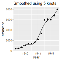
Smoothed Passenger Miles
We use a spline to smooth data on passenger miles.

quickstart.RmdThis article shows how to get started with package command. It should ideally be read in combination with the article A Workflow for Data Analysis.
command contains a single function,
cmd_assign(), which assigns objects to the global
environment. cmd_assign() can be called in two ways:
Case 2 is the important one. Case 1 is simpler, however, so we look at that first.
cmd_assign() interactively
Running
has the same effect as running
obj1 <- "orange"
obj2 <- 1
Both code snippets add two objects to the global environment, with
names "obj1" and "obj2", and values
"orange" and 1.
Objects assigned by cmd_assign() can have the following
classes:
"Hello world"
3L
3.141593
as.Date("2015-11-03")
as.POSIXct("2015-11-03 14:23:03")
as.POSIXlt("2015-11-03 14:23:03")
NULLThe objects must have length 1, except for NULL, which
has length 0.
The typical reason for using cmd_assign() interactively
is to develop code that will eventually sit in a script that is run from
the command line.
The most common way to run R scripts from the command line is with Rscript, so we take a detour to look at that.
Rscript is an application for running R scripts from the command line. For an introduction to the command line, see episodes 1–3 of The Unix Shell. For an introduction to Rscript, see Command-Line Programs.
The simplest usage is a command like
This launches a new R session, runs whatever code is in
myfile.R, and ends the session. When the session ends, all
objects in it disappear, unless they were saved to disk.
Rscript accepts additional arguments, which are placed after the path to the file being run, as in
In this example, --n_iteration=10 is a named argument,
and output.rds is an unnamed argument. Named arguments have
the format
--<name>=<value>Note that there must not be a space between the name, the
= sign, and the value, so this would be invalid:
Named arguments can also have a single dash and single letter, as in
When Rscript is called with additional arguments, Rscript supplies
the names and values for these arguments to the R session. The names and
values can be accessed from within the session using base R function commandArgs().
Working with commandArgs() is, however, tricky.
cmd_assign() is an alternative to
commandArgs(), designed specifically for workflows for data
analysis.
cmd_assign() inside a script
We will work through an example where we call
cmd_assign() inside a script that is being run from the
command line.
Our current working directory contains two files:
.
├── airmiles.csv
├── fig_smoothed.R
└── report.qmd
The file airmiles.csv holds data on annual passenger
numbers:
year,passengers
1937,412
1938,480
1939,683
1940,1052
1941,1385
1942,1418
1943,1634
1944,2178
1945,3362
1946,5948
1947,6109
1948,5981
1949,6753
1950,8003
The file fig_smoothed.R contains the following code:
## Specify packages, inputs, and outputs ------------------

suppressPackageStartupMessages({
  library(dplyr)
  library(ggplot2)
  library(command)
})

cmd_assign(.airmiles = "data/airmiles.csv",
           n_knot = 10,
           .out = "fig_smoothed.png")


## Read in data -------------------------------------------

airmiles <- read.csv(.airmiles)


## Analyse ------------------------------------------------

smoothed <- airmiles |>
  mutate(smoothed = fitted(smooth.spline(x = passengers,
                                         nknots = n_knot)))

p <- ggplot(smoothed, aes(x = year)) +
  geom_line(aes(y = smoothed)) +
  geom_point(aes(y = passengers)) +
  ggtitle(paste("Smoothed using", n_knot, "knots"))


## Save results -------------------------------------------

png(file = .out, width = 200, height = 200)
plot(p)
dev.off()
This code
.airmiles,n_knot,.out.We use Rscript to run the code from the command line.
✔ Assigned object `.airmiles` with value "airmiles.csv" and class "character".
✔ Assigned object `n_knot` with value 8 and class "numeric".
✔ Assigned object `.out` with value "fig_smoothed_8.png" and class "character".
null device
          1
Rscript started a new R session, ran the code using the command line arguments we passed in, and ended the session.
The call to cmd_assign() in fig_smoothed.R
created objects .airmiles, n_knot, and
.out inside the R session. The values for these objects
were taken from the command line, and not from the original
call to cmd_assign(). Hence, n_knot equaled
8 rather than 10, and .out
equaled "fig_smoothed_8.png" rather than
"fig_smoothed.png".
Our working directory now looks like this:
.
├── airmiles.csv
├── fig_smoothed.R
├── fig_smoothed_8.png
└── report.qmd
We have a new file called "fig_smoothed_8.png".
cmd_assign() does when called in a script
When cmd_assign() is called in a script that is being
run from the command line, it does three things:
cmd_assign().cmd_assign().Say, for instance, that we have a script called model.R
containing the following call to cmd_assign().
cmd_assign(.data = "data/dataset.csv",
           n_iter = 5,
           use_log = TRUE,
           .out = "out/model.rds")
We run model.R from the command line using
When it is first called, cmd_assign() holds the
following values:
| Argument | Value from call | Value from command line |
|---|---|---|
.data |
"data/dataset.csv" |
<none> |
n_iter |
5 |
<none> |
use_log |
TRUE |
<none> |
.out |
"out/model.rds" |
<none> |
In the match step, `cmd_assign() finds the values that were passed in from the command line. First it matches named arguments from the command line with named arguments from the call, yielding
| Argument | Value from call | Value from command line |
|---|---|---|
.data |
"data/dataset.csv" |
<none> |
n_iter |
5 |
10 |
use_log |
TRUE |
"TRUE" |
.out |
"out/model.rds" |
<none> |
Then it matches unnamed arguments from the command line with unused
arguments from the call. The matching of unnamed arguments is based on
the order in which the unnamed arguments were supplied to the command
line. In our example, the value "data/dataset2.csv" was
passed before "out/model2.rds", so
"data/dataset2.csv" comes before
"out/model2.rds" in the matched results.
| Argument | Value from call | Value from command line |
|---|---|---|
.data |
"data/dataset.csv" |
"data/dataset2.csv" |
n_iter |
5 |
"10" |
use_log |
TRUE |
"TRUE" |
.out |
"out/model.rds" |
"out/model2.rds" |
The values supplied at the command line all start out as text
strings. In the coerce step, cmd_assign()
converts these values to have the same classs as the matched values from
cmd_assign(). In our example, this means coercing
"10" to numeric and coercing
"TRUE" to logical.
| Argument | Value from call | Value from command line |
|---|---|---|
.data |
"data/dataset.csv" |
"data/dataset2.csv" |
n_iter |
5 |
10 |
use_long |
TRUE |
TRUE |
.out |
"out/model.rds" |
"out/model2.rds" |
Finally, in the assign step,
cmd_assign() puts the values into the global
environment.
The number of arguments passed through the command line must exactly
match the number of arguments specified in the call to
cmd_assign(). Values specified in the call to
cmd_assign() do not act as defaults. For instance,
in our example, cmd_assign() would not let us omit
use_log, and the following would be invalid:
In all the examples so far, the objects holding paths or filenames have conformed to a particular naming convention convention: these objects have all had names that start with a dot. For instance:
cmd_assign(.data = "data/dataset.csv", # '.data' starts with a dot
           n_iter = 5,
           use_log = TRUE,
           .out = "out/model.rds")     # '.out' starts with a dot
This idea behind the convention is to distinguish between values and
references. n_iter and use_log in the example
above hold values that are directly used in the analysis.
.data and .out, in contrast, describe were
values are stored. The distinction is analogous to the one between
ordinary variables and pointers in
C.
To access the values referred to by the “dot” variables, we use a
function such as readRDS() or read_csv(), as
in
data <- read_csv(.data)The dot-name convention is not compulsory, and
cmd_assign() does not check for it. But the convention is
nevertheless worth following, as it can be easy in practice to get
confused between a value and a reference to the value.
Another feature of the examples so far is that files with R code have
had the same base name as the files they generated as output. File
fig_smoothed.R, for instance, generated
fig_smooth.png, fig_smooth_5.png,
fig_smooth_8.png, and fig_smooth_10.png, and
file model.R generated model.rds and
model2.rds. We rely on file extensions (eg .R
vs .png) to distinguish code from outputs, and we use
suffixes (eg _5, _8 and _10) to
distinguish different versions of the same output.
Naming conventions like this are common in system programming, and are a good way to signal the relationship between code and outputs.
We can create a data analysis workflow by writing a shell script with calls to Rscript.
We illustrate with a simple example. We need two new files. The first
file, called report.qmd, creates a report with two figures.
It contains the following code.
---
title: "Smoothed Passenger Miles"
format: html
---

We use a spline to smooth data on passenger miles.

```{r}
#| label: fig_smoothed_side_by_side
#| echo: false
#| layout-ncol: 2
knitr::include_graphics(c("fig_smoothed_5.png", "fig_smoothed_10.png"))
```
The second file, called workflow.sh, is a shell script
that runs the whole workflow. It contains the following code:
Rscript fig_smoothed.R airmiles.csv 5 fig_smoothed_5.png

Rscript fig_smoothed.R airmiles.csv 10 fig_smoothed_10.png

Rscript -e "quarto::quarto_render('report.qmd')"
The third command in workflow.sh contains an
"-e" after the "Rscript". The
"-e" option tells Rscript to use code from one or more
quoted R expressions (which follow immediately after the
"-e"), rather than a file.
We run workflow.sh.
✔ Assigned object `.airmiles` with value "airmiles.csv" and class "character".
✔ Assigned object `n_knot` with value 5 and class "numeric".
✔ Assigned object `.out` with value "fig_smoothed_5.png" and class "character".
null device
          1
✔ Assigned object `.airmiles` with value "airmiles.csv" and class "character".
✔ Assigned object `n_knot` with value 10 and class "numeric".
✔ Assigned object `.out` with value "fig_smoothed_10.png" and class "character".
null device
          1


processing file: report.qmd
1/3
2/3 [fig_smoothed_side_by_side]
3/3
output file: report.knit.md

pandoc
  to: html
  output-file: report.html
  standalone: true
  section-divs: true
  html-math-method: mathjax
  wrap: none
  default-image-extension: png
  variables: {}

metadata
  document-css: false
  link-citations: true
  date-format: long
  lang: en
  title: Smoothed Passenger Miles

Output created: report.html
Our working directory now contains the two graphs and the report
(plus a directory, called report_files, created by
quarto.)
.
├── airmiles.csv
├── fig_smoothed.R
├── fig_smoothed_10.png
├── fig_smoothed_5.png
├── fig_smoothed_8.png
├── report.html
├── report.qmd
├── report_files
└── workflow.sh
The report itself looks like this:
We use a spline to smooth data on passenger miles.
An even better way to organize a data analysis workflow is to put the Rscript commands in a makefile. For an introduction to makefiles, see Project Management with Make.
Here the makefile equivalent of the workflow.sh
file:
.PHONY: all
all: report.pdf

fig_smoothed_5.png: fig_smoothed.R airmiles.csv
    Rscript $^ $@ --n_knot=5

fig_smoothed_10.png: fig_smoothed.R airmiles.csv
    Rscript $^ $@ --n_knot=10

report.pdf: report.qmd fig_smoothed_5.png fig_smoothed_10.png
    Rscript -e "quarto::quarto_render('$<')"
We delete fig_smoothed_5.png and run the makefile.
Rscript fig_smoothed.R airmiles.csv fig_smoothed_5.png --n_knot=5
✔ Assigned object `.airmiles` with value "airmiles.csv" and class "character".
✔ Assigned object `n_knot` with value 5 and class "numeric".
✔ Assigned object `.out` with value "fig_smoothed_5.png" and class "character".
null device
          1
Rscript -e "quarto::quarto_render('report.qmd')"


processing file: report.qmd
1/3
2/3 [fig_smoothed_side_by_side]
3/3
output file: report.knit.md

pandoc
  to: html
  output-file: report.html
  standalone: true
  section-divs: true
  html-math-method: mathjax
  wrap: none
  default-image-extension: png
  variables: {}

metadata
  document-css: false
  link-citations: true
  date-format: long
  lang: en
  title: Smoothed Passenger Miles

Output created: report.html
Whereas the bash script workflow.sh would have recreated
fig_smoothed_5.png, fig_smoothed_10.png and
report.html, Make recognises that
fig_smoothed_10.png is still up-to-date, so it only
recreates fig_smoothed_5.png and
report.html.
Makefiles take some time to master, but they have important advantages, discussed in A Workflow for Data Analysis.
cmd_assign()
cmd_assign() is not the only option for processing
command line arguments.
One alternative is cmdArgs()
in package R.utils,
which is a more user-friendly version of the base R function
commandArgs().
Another is package docopt, which can be used to construct an interface for script, including the processing of command line arguments.
cmd_assign() is more specialised than
cmdArgs() or docopt. It focuses
specifically on the task of processing command line arguments as part of
a data analysis workflow.