Using Package 'smoothscale'

Introduction

Package smoothscale contains functions for doing simple small area estimation with data that has sampling errors and/or measurement errors. This vignette demonstrates the use of the functions, using some synthetic data.

First we load the package.

library(smoothscale)

We will be using datasets syn_census and syn_survey.

syn_census
#> # A tibble: 100 × 5
#>    area    age   sex    child_labour all_children
#>    <chr>   <chr> <chr>         <int>        <dbl>
#>  1 Area 01 5-9   Female          134          372
#>  2 Area 02 5-9   Female           14           35
#>  3 Area 03 5-9   Female           92          388
#>  4 Area 04 5-9   Female           46          345
#>  5 Area 05 5-9   Female           25          102
#>  6 Area 06 5-9   Female            2            5
#>  7 Area 07 5-9   Female            4           13
#>  8 Area 08 5-9   Female           10           34
#>  9 Area 09 5-9   Female            2           52
#> 10 Area 10 5-9   Female          578         2087
#> # ℹ 90 more rows

The datasets contains synthetic (i.e. fake) data, but the data has a similar structure to real census and survey data. syn_census contains, for each combination of area, age, and sex, counts of children involved in child labour, and counts of all children. syn_survey contains estimates of overall probabilities of being involved in child labour, which are assumed to be accurate.

Function `smooth_prob()`

Function smooth_prob() deals with sampling error, which is typically an important problem when doing small area estimation. Function smooth_prob() has two main arguments:

count is the count variable that needs to be smoothed, in our case, counts of child labour
size is the number of respondents from which counts were draw, in our case, counts of all children in the census file.

A ‘direct’ estimate of the probability that a child is involved in child labour can be produced by simply dividing each area’s count of child labour by the number of children,

direct <- syn_census$child_labour / syn_census$all_children
summary(direct)
#>    Min. 1st Qu.  Median    Mean 3rd Qu.    Max. 
#>  0.0000  0.1885  0.2500  0.2651  0.3170  0.8000

A smoothed version of these estimates can be produced using function smooth_prob():

smoothed <- smooth_prob(x = syn_census$child_labour,
                        size = syn_census$all_children)
summary(smoothed)
#>    Min. 1st Qu.  Median    Mean 3rd Qu.    Max. 
#>  0.1053  0.2137  0.2537  0.2645  0.2978  0.5186

Function smooth_prob() pulls prevalences (ie counts divided by size) towards the overall average. We know, however, that child labour is likely to vary by age and sex. It would be better to smooth each combination of age and sex towards their own average.

A convenient way to smooth within combinations of other variables is to use functions contained in the dplyr package (part of thetidyverse.)

library(dplyr)
#> 
#> Attaching package: 'dplyr'
#> The following objects are masked from 'package:stats':
#> 
#>     filter, lag
#> The following objects are masked from 'package:base':
#> 
#>     intersect, setdiff, setequal, union
smoothed_agesex <- syn_census |>
  group_by(age, sex) |>
  mutate(direct = child_labour / all_children,
         smoothed = smooth_prob(x = child_labour,
                                size = all_children)) |>
  ungroup()
smoothed_agesex
#> # A tibble: 100 × 7
#>    area    age   sex    child_labour all_children direct smoothed
#>    <chr>   <chr> <chr>         <int>        <dbl>  <dbl>    <dbl>
#>  1 Area 01 5-9   Female          134          372 0.360    0.351 
#>  2 Area 02 5-9   Female           14           35 0.4      0.325 
#>  3 Area 03 5-9   Female           92          388 0.237    0.236 
#>  4 Area 04 5-9   Female           46          345 0.133    0.140 
#>  5 Area 05 5-9   Female           25          102 0.245    0.241 
#>  6 Area 06 5-9   Female            2            5 0.4      0.252 
#>  7 Area 07 5-9   Female            4           13 0.308    0.252 
#>  8 Area 08 5-9   Female           10           34 0.294    0.264 
#>  9 Area 09 5-9   Female            2           52 0.0385   0.0995
#> 10 Area 10 5-9   Female          578         2087 0.277    0.276 
#> # ℹ 90 more rows

We calculate and plot prevalences, using some more tidyverse packages and functions,

library(tidyr)
library(forcats)
library(ggplot2)
data_for_plot <- smoothed_agesex |>
  pivot_longer(col = c(direct, smoothed),
               names_to = "measure",
                 values_to = "prob") |>
  mutate(area = fct_reorder(area, prob))
ggplot(data_for_plot,
       aes(x = prob, y = area, color = measure)) +
  facet_grid(vars(age), vars(sex)) +
  geom_point() +
  scale_color_manual(values = c("darkblue", "darkorange"))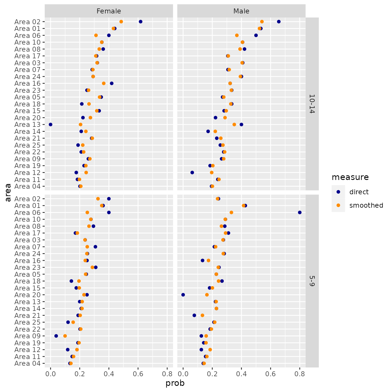

Function `scale_prob()`

Function scale_prob() deals with measurement error, which also arises often in small area estimation. Function scale_prob() has three arguments:

unscaled is the original probability estimate for each area
benchmark is an overall probability, assumed to be error-free
wt is an optional weighting variable, used to calculate an overall probability from unscaled.

We can use scale_prob() to scale the probabilities estimated earlier using smooth_prob() so that they match those from syn_survey at the national level.

scaled_agesex <- smoothed_agesex |>
  inner_join(syn_survey) |>
  group_by(age, sex) |>
  mutate(scaled = scale_prob(unscaled = smoothed,
                             benchmark = prob_child_labour)) %>%
  ungroup()
#> Joining with `by = join_by(age, sex)`
scaled_agesex 
#> # A tibble: 100 × 9
#>    area  age   sex   child_labour all_children direct smoothed prob_child_labour
#>    <chr> <chr> <chr>        <int>        <dbl>  <dbl>    <dbl>             <dbl>
#>  1 Area… 5-9   Fema…          134          372 0.360    0.351              0.297
#>  2 Area… 5-9   Fema…           14           35 0.4      0.325              0.297
#>  3 Area… 5-9   Fema…           92          388 0.237    0.236              0.297
#>  4 Area… 5-9   Fema…           46          345 0.133    0.140              0.297
#>  5 Area… 5-9   Fema…           25          102 0.245    0.241              0.297
#>  6 Area… 5-9   Fema…            2            5 0.4      0.252              0.297
#>  7 Area… 5-9   Fema…            4           13 0.308    0.252              0.297
#>  8 Area… 5-9   Fema…           10           34 0.294    0.264              0.297
#>  9 Area… 5-9   Fema…            2           52 0.0385   0.0995             0.297
#> 10 Area… 5-9   Fema…          578         2087 0.277    0.276              0.297
#> # ℹ 90 more rows
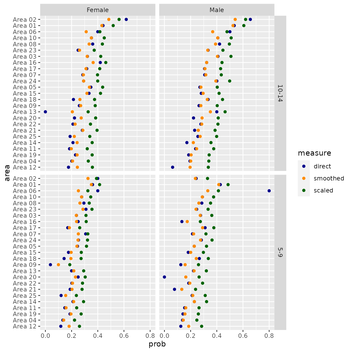
#> # ℹ 1 more variable: scaled <dbl>

We graph the results.

data_for_plot_scaled <- scaled_agesex |>
  pivot_longer(col = c(direct, smoothed, scaled),
               names_to = "measure",
                 values_to = "prob") |>
  mutate(measure = factor(measure, levels = c("direct", "smoothed", "scaled")),
         area = fct_reorder(area, prob))
ggplot(data_for_plot_scaled,
       aes(x = prob, y = area, color = measure)) +
  facet_grid(vars(age), vars(sex)) +
  geom_point() +
  scale_color_manual(values = c("darkblue", "darkorange", "darkgreen"))

Introduction

Function smooth_prob()

Function scale_prob()

Function `smooth_prob()`

Function `scale_prob()`