Priors

1 Set-up

suppressPackageStartupMessages({
  library(bage)
  library(poputils)
  library(ggplot2)
  library(dplyr)
})

plot_exch <- function(draws) {
  ggplot(draws, aes(x = element, y = value)) +
    facet_wrap(vars(draw), nrow = 1) +
    geom_hline(yintercept = 0, col = "grey") +
    geom_point(col = "darkblue", size = 0.7) +
    scale_x_continuous(n.breaks = max(draws$element)) +
    xlab("Unit") +
    ylab("") +
    theme(text = element_text(size = 8))
}

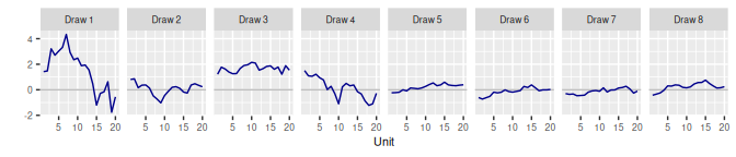
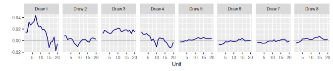
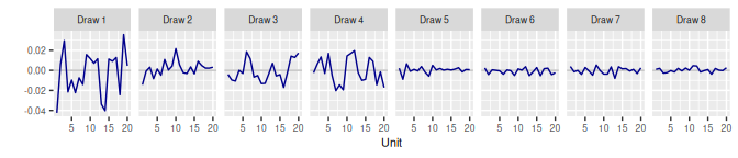
plot_cor_one <- function(draws) {
  ggplot(draws, aes(x = along, y = value)) +
    facet_wrap(vars(draw), nrow = 1) +
    geom_hline(yintercept = 0, col = "grey") +
    geom_line(col = "darkblue") +
    xlab("Unit") +
    ylab("") +
    theme(text = element_text(size = 8))
}

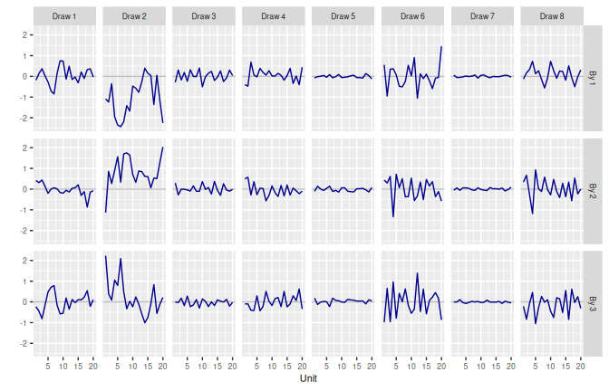
plot_cor_many <- function(draws) {
  ggplot(draws, aes(x = along, y = value)) +
    facet_grid(vars(by), vars(draw)) +
    geom_hline(yintercept = 0, col = "grey") +
    geom_line(col = "darkblue") +
    xlab("Unit") +
    ylab("") +
    theme(text = element_text(size = 8))
}

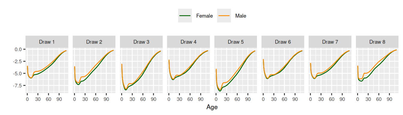
plot_svd_one <- function(draws) {
  ggplot(draws, aes(x = age_mid(age), y = value, color = sex)) +
    facet_wrap(vars(draw), nrow = 1) +
    geom_line() +
    scale_color_manual(values = c("darkgreen", "darkorange")) +
    xlab("Age") +
    ylab("") +
    theme(text = element_text(size = 8),
          legend.position = "top",
          legend.title = element_blank())
}

plot_svd_many <- function(draws) {
  draws |>
    mutate(element = paste("Unit", element)) |>
    ggplot(aes(x = age_mid(age), y = value, color = sex)) +
    facet_grid(vars(element), vars(draw)) +
    geom_line() +
    scale_color_manual(values = c("darkgreen", "darkorange")) +
    xlab("Age") +
    ylab("") +
    theme(text = element_text(size = 8),
          legend.position = "top",
          legend.title = element_blank())
}

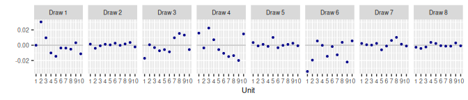
2 Exchangeable Units

2.1 Fixed Normal `NFix()`

2.1.1 Model

\[\begin{equation} \beta_j \sim \text{N}(0, \mathtt{sd}^2) \end{equation}\]

Defaults:

sd: 1

2.1.2 Examples

All defaults

set.seed(0)

NFix() |>
  generate(n_element = 10, n_draw = 8) |>
  plot_exch()

Reduce `sd`

set.seed(0)

NFix(sd = 0.01) |>
  generate(n_element = 10, n_draw = 8) |>
  plot_exch()

2.2 Normal `N()`

2.2.1 Model

\[\begin{align} \beta_j & \sim \text{N}(0, \tau^2) \\ \tau & \sim \text{N}^+(0, \mathtt{s}) \end{align}\]

Defaults:

s: 1

2.2.2 Examples

All defaults

set.seed(0)

N() |>
  generate(n_element = 10, n_draw = 8) |>
  plot_exch()

Reduce `s`

set.seed(0)

N(s = 0.01) |>
  generate(n_element = 10, n_draw = 8) |>
  plot_exch()

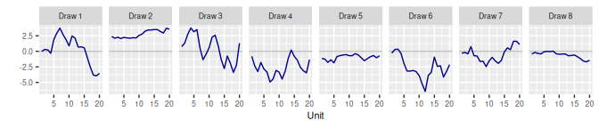
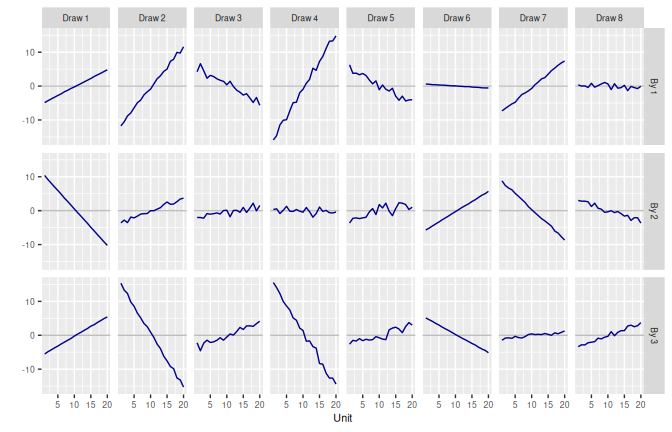
3 Units Correlated With Neighbours

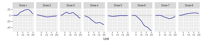
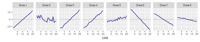
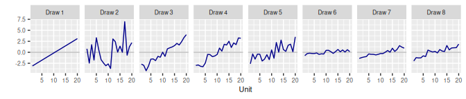
3.1 Random Walk `RW()`

3.1.1 Model

\[\begin{align} \beta_1 & \sim \text{N}(0, \mathtt{sd}^2) \\ \beta_j & \sim \text{N}(\beta_{j-1}, \tau^2), \quad j = 2, \cdots, J \\ \tau & \sim \text{N}^+(0, \mathtt{s}^2) \end{align}\]

Defaults:

s: 1
sd: 1

3.1.2 Examples

All defaults

set.seed(0)

RW() |>
  generate(n_draw = 8) |>
  plot_cor_one()

Reduce `s`

set.seed(0)

RW(s = 0.01) |>
  generate(n_draw = 8) |>
  plot_cor_one()

Reduce `s` and `sd`

set.seed(0)

RW(s = 0.01, sd = 0) |>
  generate(n_draw = 8) |>
  plot_cor_one()

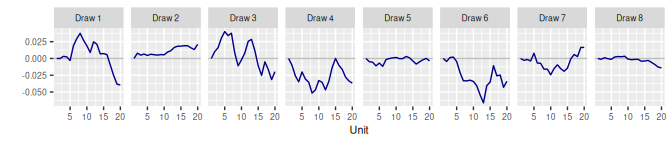
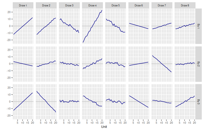
3.2 Second-Order Random Walk `RW2()`

3.2.1 Model

\[\begin{align} \beta_1 & \sim \text{N}(0, \mathtt{sd}^2) \\ \beta_2 & \sim \text{N}(\beta_1, \mathtt{sd\_slope}^2) \\ \beta_j & \sim \text{N}(2\beta_{j-1} - \beta_{j-2}, \tau^2), \quad j = 3, \cdots, J \\ \tau & \sim \text{N}^+(0, \mathtt{s}^2) \end{align}\]

Defaults:

s: 1
sd: 1
sd_slope: 1

3.2.2 Examples

All defaults

set.seed(0)

RW2() |>
  generate(n_draw = 8) |>
  plot_cor_one()

Reduce `s`

set.seed(0)

RW2(s = 0.01) |>
  generate(n_draw = 8) |>
  plot_cor_one()

Reduce `s` and `sd_slope`

set.seed(0)

RW2(s = 0.01, sd_slope = 0.01) |>
  generate(n_draw = 8) |>
  plot_cor_one()

Reduce `s`, `sd`, and `sd_slope`

set.seed(0)

RW2(s = 0.01, sd = 0, sd_slope = 0.01) |>
  generate(n_draw = 8) |>
  plot_cor_one()

3.3 Autoregressive `AR()`

3.3.1 Model

\[\begin{equation} \beta_j \sim \text{N}\left(\phi_1 \beta_{j-1} + \cdots + \phi_{\mathtt{n\_coef}} \beta_{j-\mathtt{n\_coef}}, \omega^2\right) \end{equation}\] TMB derives a value of \(\omega\) that gives each \(\beta_j\) variance \(\tau^2\). The prior for \(\tau\) is \[\begin{equation} \tau \sim \text{N}^+(0, \mathtt{s}^2). \end{equation}\] The prior for each \(\phi_k\) is \[\begin{equation} \frac{\phi_k + 1}{2} \sim \text{Beta}(\mathtt{shape1}, \mathtt{shape2}). \end{equation}\]

Defaults:

-n_coef: 2 - s: 1

3.3.2 Examples

All defaults

set.seed(0)

AR() |>
  generate(n_draw = 8) |>
  plot_cor_one()

Increase `n_coef`

set.seed(0)

AR(n_coef = 3) |>
  generate(n_draw = 8) |>
  plot_cor_one()

Reduce `s`

set.seed(0)

AR(s = 0.01) |>
  generate(n_draw = 8) |>
  plot_cor_one()

Specify ‘along’ and ‘by’ dimensions

set.seed(0)

AR() |>
  generate(n_along = 20, n_by = 3, n_draw = 8) |>
  plot_cor_many()

Specify ‘along’ and ‘by’ dimensions, set `con = "by"`

set.seed(0)

AR(con = "by") |>
  generate(n_along = 20, n_by = 3, n_draw = 8) |>
  plot_cor_many()

3.4 First-Order Autoregressive `AR1()`

3.4.1 Model

\[\begin{equation} \beta_j \sim \text{N}\left(\phi \beta_{j-1}, \omega^2\right) \end{equation}\] TMB derives a value of \(\omega\) that gives each \(\beta_j\) variance \(\tau^2\). The prior for \(\tau\) is \[\begin{equation} \tau \sim \text{N}^+(0, \mathtt{s}^2). \end{equation}\] The prior for \(\phi\) is \[\begin{equation} \frac{\phi - \mathtt{min}}{\mathtt{max} - \mathtt{min}} \sim \text{Beta}(\mathtt{shape1}, \mathtt{shape2}). \end{equation}\]

Defaults:

s: 1
min: 0.8
max: 0.98

3.4.2 Examples

All defaults

set.seed(0)

AR1() |>
  generate(n_draw = 8) |>
  plot_cor_one()

Reduce `s`

set.seed(0)

AR1(s = 0.01) |>
  generate(n_draw = 8) |>
  plot_cor_one()

Reduce `s` and modify `min`, `max`

set.seed(0)

AR1(s = 0.01, min = -1, max = 1) |>
  generate(n_draw = 8) |>
  plot_cor_one()

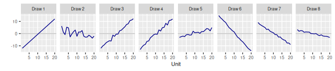
4 Curves

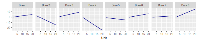
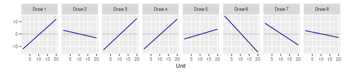
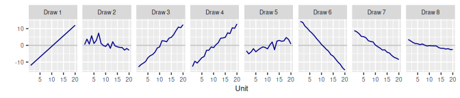
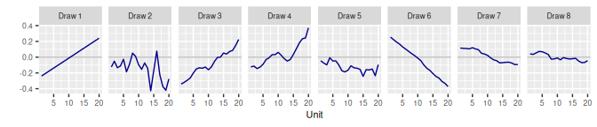
4.1 Linear `Lin()`

4.1.1 Model

Default:

s: 1
mean_slope: 0
sd_slope: 1

4.1.2 Examples

All defaults

set.seed(0)

Lin() |>
  generate(n_draw = 8) |>
  plot_cor_one()

Reduce `s`

s = 0, mean_slope = 0, sd_slope = 1

set.seed(0)

Lin(s = 0) |>
  generate(n_draw = 8) |>
  plot_cor_one()

Modify `mean_slope`, `sd_slope`

s = 1, mean_slope = 0.2, sd_slope = 0.1

set.seed(0)

Lin(mean_slope = 0.2, sd_slope = 0.1) |>
  generate(n_draw = 8) |>
  plot_cor_one()

Specify ‘along’ and ‘by’ dimensions

set.seed(0)

Lin() |>
  generate(n_along = 20, n_by = 3, n_draw = 8) |>
  plot_cor_many()

Specify ‘along’ and ‘by’ dimensions, set `con = "by"`

set.seed(0)

Lin(con = "by") |>
  generate(n_along = 20, n_by = 3, n_draw = 8) |>
  plot_cor_many()

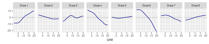
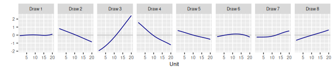
4.2 Penalised Spline `Sp()`

4.2.1 Model

\[\begin{align} \pmb{\beta} & = \bm{X} \pmb{\alpha} \\ \alpha_1 & \sim \text{N}(0, \mathtt{sd}^2) \\ \alpha_2 & \sim \text{N}(\alpha_1, \mathtt{sd\_slope}^2) \\ \alpha_j & \sim \text{N}(2\alpha_{j-1} - \alpha_{j-2}, \tau^2), \quad j = 3, \cdots, J \\ \tau & \sim \text{N}^+\left(0, \mathtt{s}^2\right) \\ \end{align}\]

Defaults

n_comp: NULL
s: 1
sd: 1
sd_slope: 1

All defaults

set.seed(0)

Sp() |>
  generate(n_draw = 8) |>
  plot_cor_one()

Specify `n_comp`

set.seed(0)

Sp(n_comp = 5) |>
  generate(n_draw = 8) |>
  plot_cor_one()

Reduce `s`, `sd`, `sd_slope`

set.seed(0)

Sp(s = 0.01, sd = 0.01, sd_slope = 0.01) |>
  generate(n_draw = 8) |>
  plot_cor_one()

5 Composite Priors

5.1 Second Order Random Walk with Autoregressive Errors `RW2_AR()`

5.1.1 Model

\[\begin{align} \beta_j & = \alpha_j + \epsilon_j \\ \alpha_1 & \sim \text{N}(0, \mathtt{sd}^2) \\ \alpha_2 & \sim \text{N}(\alpha_1, \mathtt{sd\_slope}^2) \\ \alpha_j & \sim \text{N}(2\alpha_{j-1} - \alpha_{j-2}, \tau^2), \quad j = 3, \cdots, J \\ \tau & \sim \text{N}^+(0, \mathtt{s}^2) \\ \epsilon_j & \sim \text{N}\left(\phi_1 \epsilon_{j-1} + \cdots + \phi_{\mathtt{n\_coef}} \epsilon_{j-\mathtt{n\_coef}}, \omega^2\right) \\ \tau & \sim \text{N}^+\left(0, \mathtt{s}^2\right) \\ \frac{\phi_k + 1}{2} & \sim \text{Beta}(\mathtt{shape1}, \mathtt{shape2}) \end{align}\]

Defaults:

s_rw: 1
sd: 1
sd_slope: 1
n_coef: 2
s_ar: 1
shape1: 5
shape2: 5

5.1.2 Examples

All defaults

set.seed(0)

RW2_AR() |>
  generate(n_draw = 8) |>
  plot_cor_one()

Reduce `s_rw`, `s`, `sd_slope`

set.seed(0)

RW2_AR(s_rw = 0.1, sd = 0.1, sd_slope = 0.1) |>
  generate(n_draw = 8) |>
  plot_cor_one()

Reduce `s_ar`

set.seed(0)

RW2_AR(s_ar = 0.1) |>
  generate(n_draw = 8) |>
  plot_cor_one()

5.2 Second Order Random Walk with First Order Autoregressive Errors `RW2_AR1()`

5.2.1 Model

TMB derives a value of \(\omega\) that gives each \(\epsilon_j\) variance \(\tau^2\). The prior for \(\tau\) is \[\begin{equation} \tau \sim \text{N}^+(0, \mathtt{s}^2). \end{equation}\] The prior for \(\phi\) is \[\begin{equation} \frac{\phi - \mathtt{min}}{\mathtt{max} - \mathtt{min}} \sim \text{Beta}(\mathtt{shape1}, \mathtt{shape2}). \end{equation}\]

Defaults:

s_rw: 1
sd: 1
sd_slope: 1
s_ar: 1
shape1: 5
shape2: 5
min: 0.8
max: 0.98

5.2.2 Examples

All defaults

set.seed(0)

RW2_AR1() |>
  generate(n_draw = 8) |>
  plot_cor_one()

Reduce `s_rw`, `s`, `sd_slope`

set.seed(0)

RW2_AR1(s_rw = 0.1, sd = 0.1, sd_slope = 0.1) |>
  generate(n_draw = 8) |>
  plot_cor_one()

Reduce `s_ar`

set.seed(0)

RW2_AR1(s_ar = 0.1) |>
  generate(n_draw = 8) |>
  plot_cor_one()

5.3 Linear with AR Errors `Lin_AR()`

5.3.1 Model

\[\begin{align} \beta_j & = \alpha_j + \epsilon_j \\ \alpha_j & = \left(j - \frac{J + 1}{2}\right) \eta \\ \eta & \sim \text{N}\left(\mathtt{mean\_slope}, \mathtt{sd\_slope}^2 \right) \\ \epsilon_j & \sim \text{N}\left(\phi_1 \epsilon_{j-1} + \cdots + \phi_{\mathtt{n\_coef}} \epsilon_{j-\mathtt{n\_coef}}, \omega^2\right) \tau & \sim \text{N}^+\left(0, \mathtt{s}^2\right) \\ \frac{\phi_k + 1}{2} & \sim \text{Beta}(\mathtt{shape1}, \mathtt{shape2}) \end{align}\]

Defaults:

n_coef: 2
s: 1
mean_slope: 0
sd_slope: 1

5.3.2 Examples

All defaults

set.seed(0)

Lin_AR() |>
  generate(n_draw = 8) |>
  plot_cor_one()

5.3.2.1 Reduce `s`, `sd_slope`

set.seed(0)

Lin_AR(s = 0.1, sd_slope = 0.01) |>
  generate(n_draw = 8) |>
  plot_cor_one()

5.4 Linear with AR1 Errors `Lin_AR1()`

5.4.1 Model

\[\begin{align} \beta_j & = \alpha_j + \epsilon_j \\ \alpha_j & = \left(j - \frac{J + 1}{2}\right) \eta \\ \eta & \sim \text{N}\left(\mathtt{mean\_slope}, \mathtt{sd\_slope}^2 \right) \\ \epsilon_j & \sim \text{N}\left(\phi \epsilon_{j-1}, \omega^2\right) \tau & \sim \text{N}^+\left(0, \mathtt{s}^2\right) \\ \frac{\phi - \mathtt{min}}{\mathtt{max} - \mathtt{min}} \sim \text{Beta}(\mathtt{shape1}, \mathtt{shape2}) \end{align}\]

Defaults:

s: 1
min: 0.8
max: 0.98
mean_slope: 0
sd_slope: 1

5.4.2 Examples

All defaults

set.seed(0)

Lin_AR1() |>
  generate(n_draw = 8) |>
  plot_cor_one()

5.4.2.1 Modify `min`, `max`

set.seed(0)

Lin_AR1(min = -1, max = 1) |>
  generate(n_draw = 8) |>
  plot_cor_one()

5.4.2.2 Reduce `s`, `sd_slope`

set.seed(0)

Lin_AR1(s = 0.1, sd_slope = 0.02) |>
  generate(n_draw = 8) |>
  plot_cor_one()

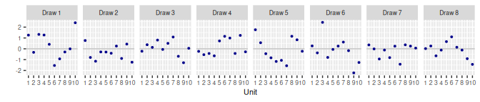
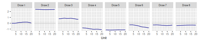
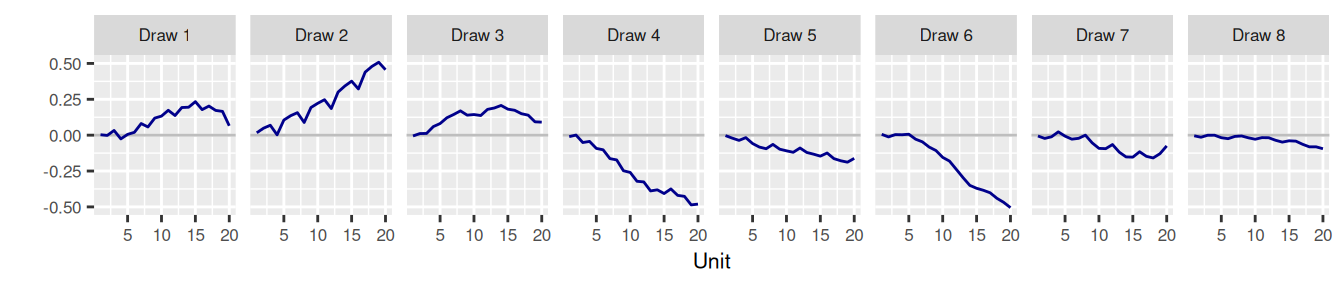
5.5 Random Walk with Seasonal Effects `RW_Seas()`

5.5.1 Model

\[\begin{align} \beta_j & = \alpha_j + \lambda_j \\ \alpha_1 & \sim \text{N}(0, \mathtt{sd}^2) \\ \alpha_j & \sim \text{N}(\alpha_{j-1}, \tau^2), \quad j = 2, \cdots, J \\ \tau & \sim \text{N}^+\left(0, \mathtt{s}^2\right) \\ \lambda_j & \sim \text{N}(0, \mathtt{sd\_seas}^2), \quad j = 1, \cdots, \mathtt{n\_seas} - 1 \\ \lambda_j & = -\sum_{s=1}^{j-1} \lambda_{j-s}, \quad j = \mathtt{n\_seas},\; 2 \mathtt{n\_seas}, \cdots \\ \lambda_j & \sim \text{N}(\lambda_{j-\mathtt{n\_seas}}, \omega^2), \quad \text{otherwise} \\ \omega & \sim \text{N}^+\left(0, \mathtt{s\_seas}^2\right) \end{align}\]

Defaults:

s: 1
sd: 1
sd_seas: 1
s_seas: 0

All defaults plus `s_seas = 0`

set.seed(0)

RW_Seas(n_seas = 4, s_seas = 0) |>
  generate(n_draw = 8) |>
  plot_cor_one()

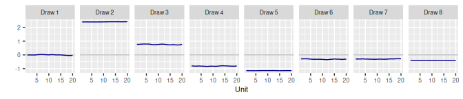
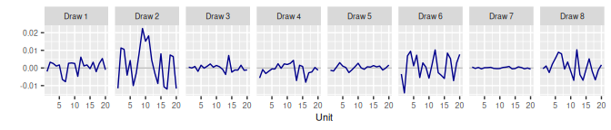
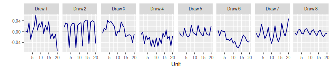
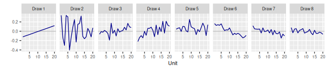
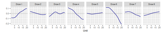
5.5.1.1 Reduce `s`, `sd`

set.seed(0)

RW_Seas(n_seas = 4, s = 0.01, sd = 0, s_seas = 0) |>
  generate(n_draw = 8) |>
  plot_cor_one()

5.5.1.2 Non-zero `s_seas`

set.seed(0)

RW_Seas(n_seas = 4, s = 0.01, sd = 0, s_seas = 1) |>
  generate(n_draw = 8) |>
  plot_cor_one()

5.5.1.3 Reduce `sd_seas`

set.seed(0)

RW_Seas(n_seas = 4, s = 0.01, sd = 0, s_seas = 0, sd_seas = 0.01) |>
  generate(n_draw = 8) |>
  plot_cor_one()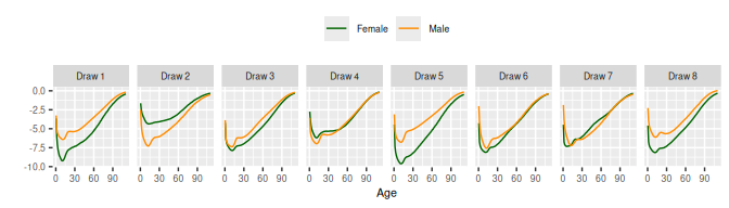

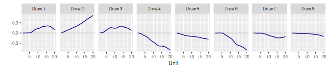
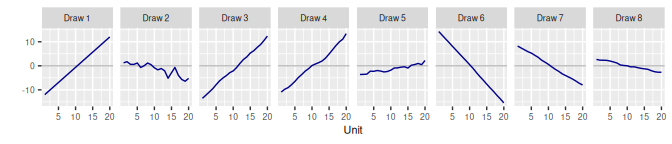
5.6 Second-Order Random Walk with Seasonal Effects `RW2_Seas()`

5.6.1 Model

\[\begin{align} \beta_j & = \alpha_j + \lambda_j \\ \alpha_1 & \sim \text{N}(0, \mathtt{sd}^2) \\ \alpha_2 & \sim \text{N}(\alpha_1, \mathtt{sd\_slope}^2) \\ \alpha_j & \sim \text{N}(2\alpha_{j-1} - \alpha_{j-2}, \tau^2), \quad j = 3, \cdots, J \\ \tau & \sim \text{N}^+\left(0, \mathtt{s}^2\right) \\ \lambda_j & \sim \text{N}(0, \mathtt{sd\_seas}^2), \quad j = 1, \cdots, \mathtt{n\_seas} - 1 \\ \lambda_j & = -\sum_{s=1}^{j-1} \lambda_{j-s}, \quad j = \mathtt{n\_seas},\; 2 \mathtt{n\_seas}, \cdots \\ \lambda_j & \sim \text{N}(\lambda_{j-\mathtt{n\_seas}}, \omega^2), \quad \text{otherwise} \\ \omega & \sim \text{N}^+\left(0, \mathtt{s\_seas}^2\right) \end{align}\]

Defaults:

s: 1
sd: 1
sd_slope: 1
s_seas: 0
sd_seas: 1

5.6.2 Examples

5.6.2.1 All defaults {-}, plus `s_seas = 0`

set.seed(0)

RW2_Seas(n_seas = 4, s_seas = 0) |>
  generate(n_draw = 8) |>
  plot_cor_one()

5.6.2.2 Reduce `s`, `sd`, `sd_slope`, `sd_seas`

set.seed(0)

RW2_Seas(n_seas = 4, s = 0.01, sd = 0, sd_slope = 0.01,
         s_seas = 0, sd_seas = 0.01) |>
  generate(n_draw = 8) |>
  plot_cor_one()

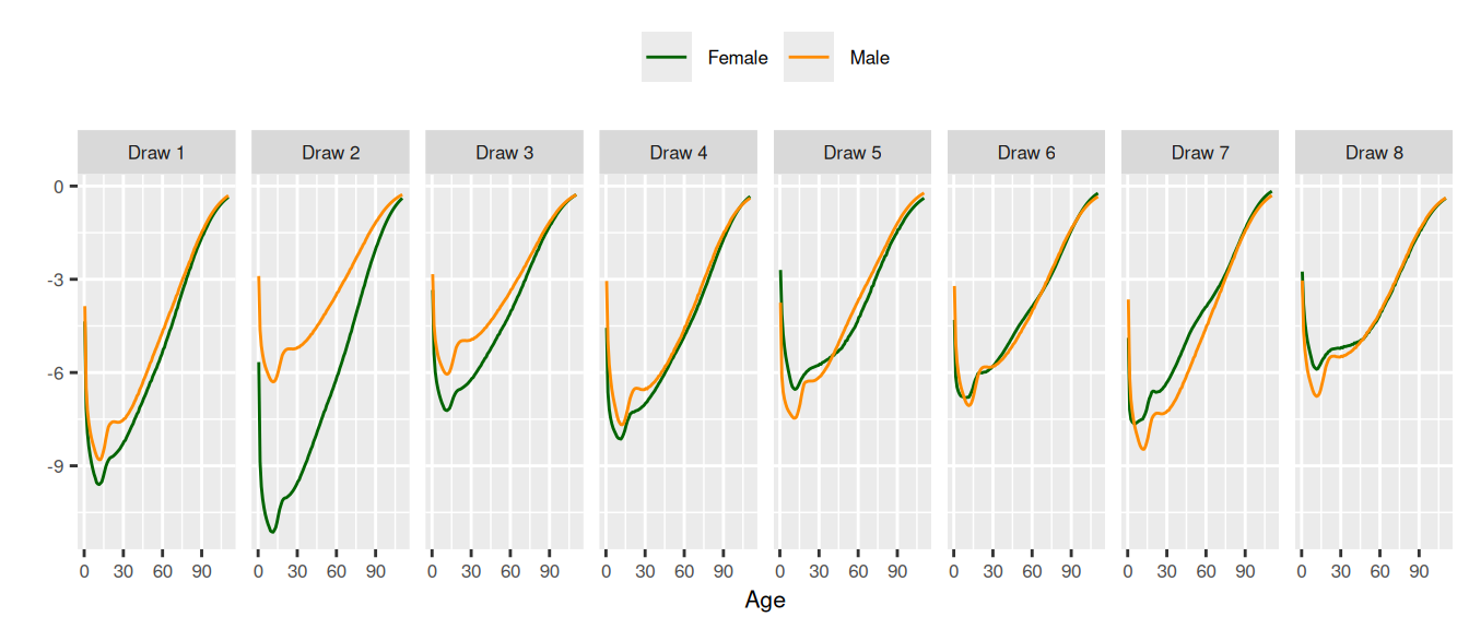
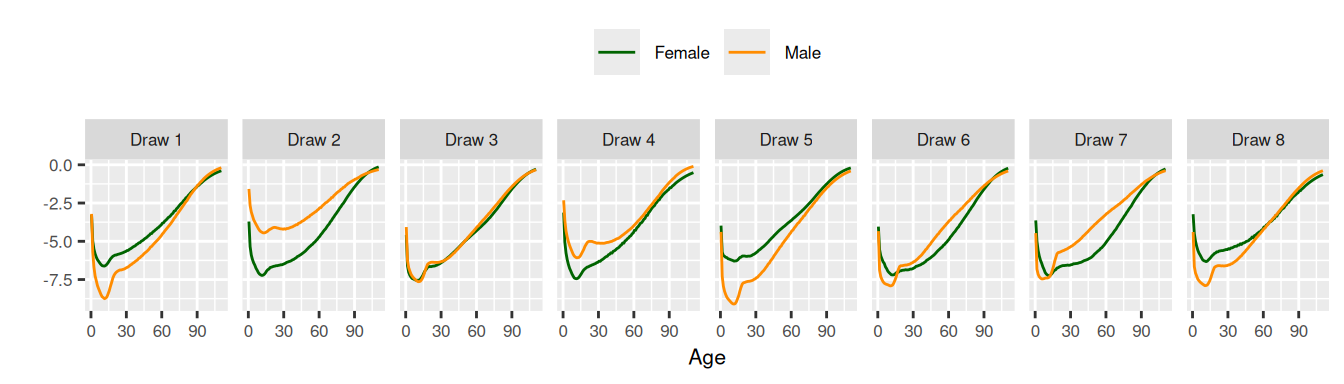
6 SVD-Based Priors

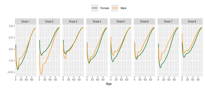
6.1 Exchangeable `SVD()`

6.1.1 Model

\[\begin{equation} \pmb{\beta} = \pmb{F} \pmb{\alpha} + \pmb{g} \end{equation}\]

Defaults:

n_comp: NULL
indep: TRUE

6.1.2 Experiments

All defaults

set.seed(0)

SVD(HMD) |>
  generate(n_draw = 8) |>
  plot_svd_one()

6.1.2.1 Increase `n_comp`

SVD(HMD, n_comp = 5) |>
  generate(n_draw = 8) |>
  plot_svd_one()

6.1.2.2 Set `indep` to `FALSE`

SVD(HMD, indep = FALSE) |>
  generate(n_draw = 8) |>
  plot_svd_one()

6.1.2.3 Multiple units

SVD(HMD, indep = FALSE) |>
  generate(n_draw = 8, n_element = 3) |>
  plot_svd_many()

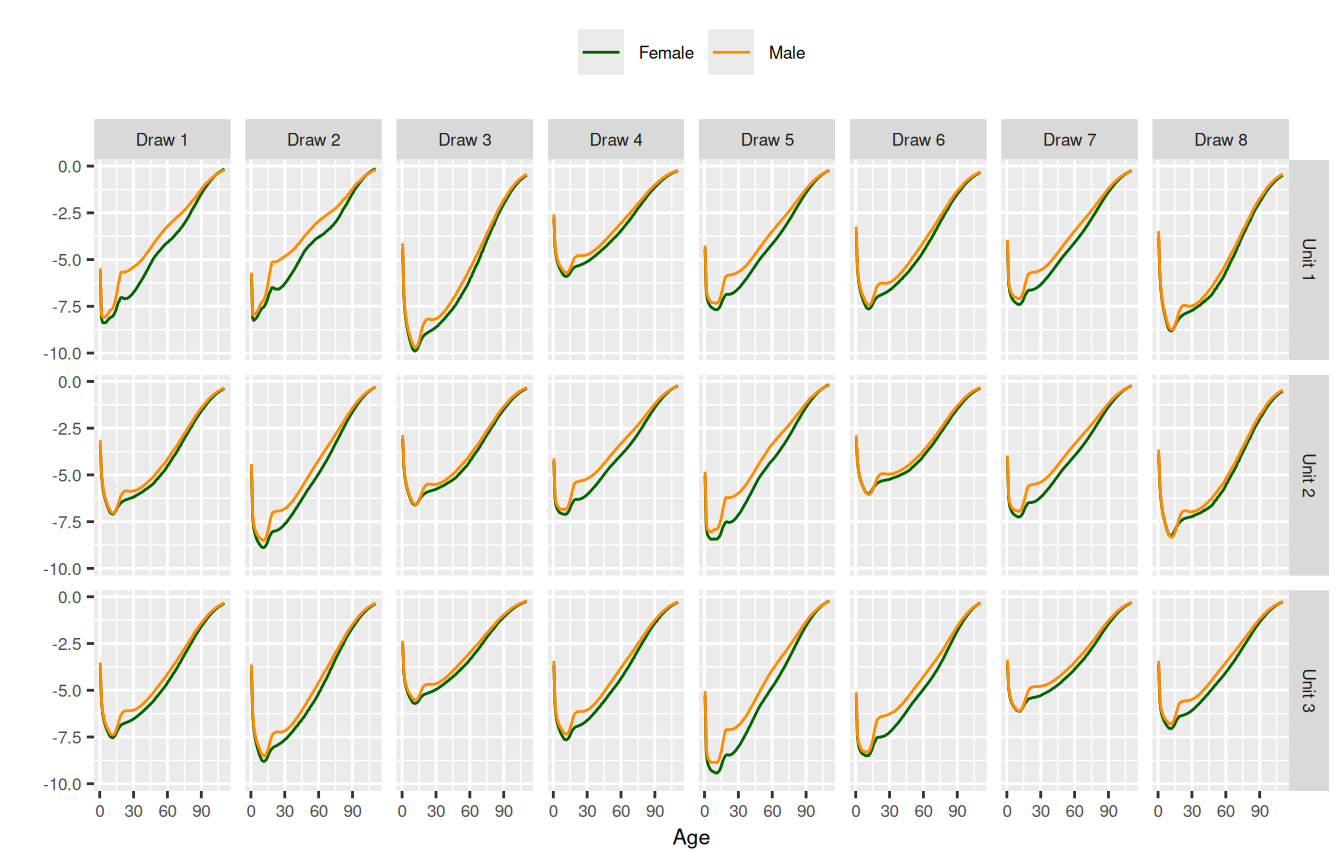
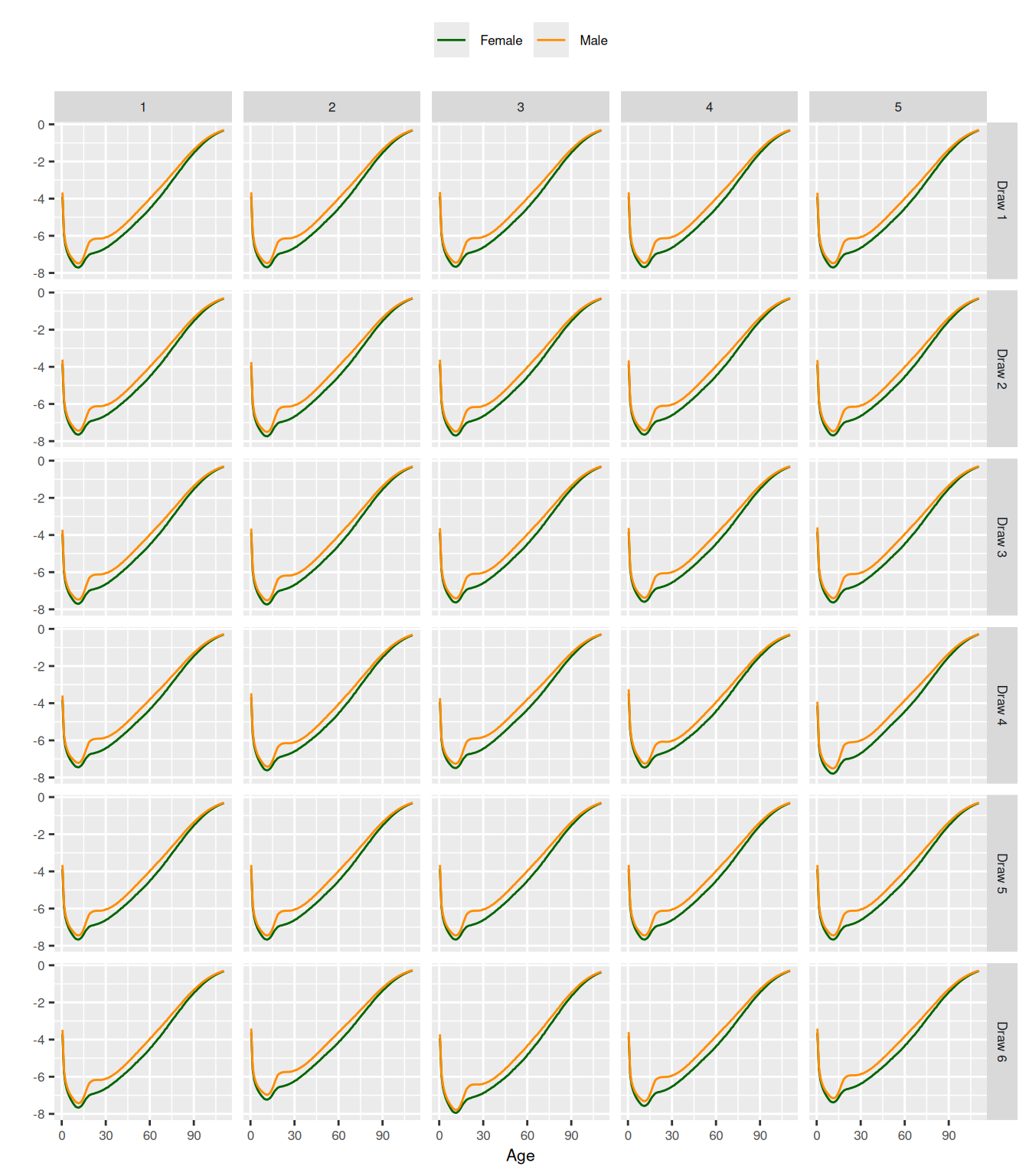
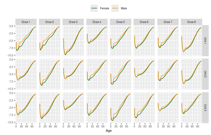
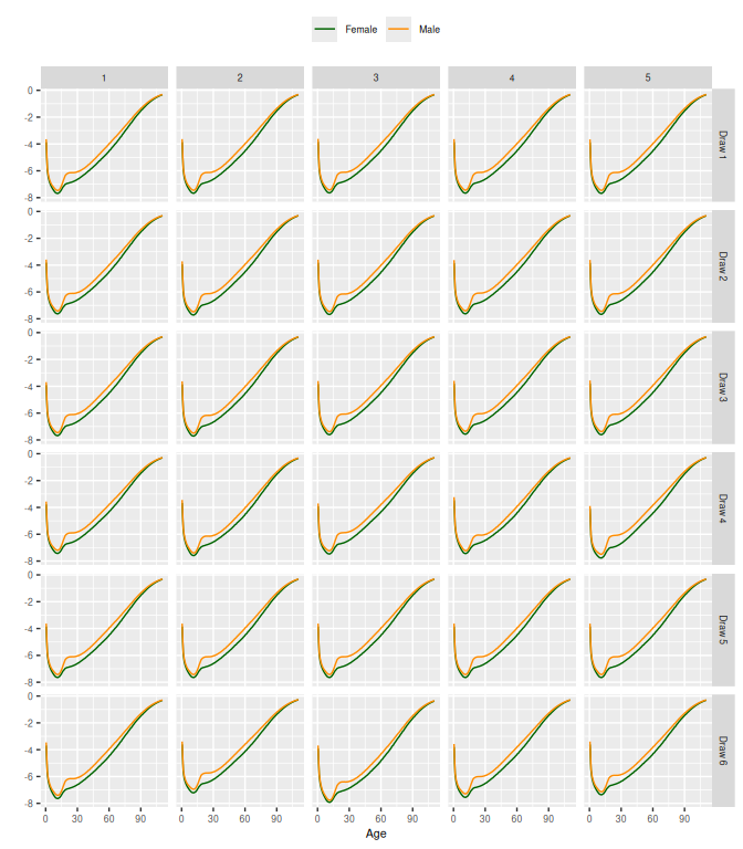
6.2 Dynamic SVD Prior with Autoregressive Weights `SVD_AR()`

6.2.1 Model

SVD_AR(HMD, indep = FALSE, s = 0.1) |>
  generate(n_draw = 6, n_along = 5) |>
    ggplot(aes(x = age_mid(age), 
                      y = value, 
                      color = sex)) +
      facet_grid(vars(draw), vars(along)) +
      geom_line() +
      scale_color_manual(values = c("darkgreen", "darkorange")) +
      xlab("Age") +
      ylab("") +
      theme(text = element_text(size = 8),
            legend.position = "top",
            legend.title = element_blank())

1 Set-up

2 Exchangeable Units

2.1 Fixed Normal NFix()

2.1.1 Model

2.1.2 Examples

All defaults

Reduce sd

2.2 Normal N()

2.2.1 Model

2.2.2 Examples

All defaults

Reduce s

3 Units Correlated With Neighbours

3.1 Random Walk RW()

3.1.1 Model

3.1.2 Examples

All defaults

Reduce s

Reduce s and sd

3.2 Second-Order Random Walk RW2()

3.2.1 Model

3.2.2 Examples

All defaults

Reduce s

Reduce s and sd_slope

Reduce s, sd, and sd_slope

3.3 Autoregressive AR()

3.3.1 Model

3.3.2 Examples

All defaults

Increase n_coef

Reduce s

Specify ‘along’ and ‘by’ dimensions

Specify ‘along’ and ‘by’ dimensions, set con = "by"

3.4 First-Order Autoregressive AR1()

3.4.1 Model

3.4.2 Examples

All defaults

Reduce s

Reduce s and modify min, max

4 Curves

4.1 Linear Lin()

4.1.1 Model

4.1.2 Examples

All defaults

Reduce s

Modify mean_slope, sd_slope

Specify ‘along’ and ‘by’ dimensions

Specify ‘along’ and ‘by’ dimensions, set con = "by"

4.2 Penalised Spline Sp()

4.2.1 Model

All defaults

Specify n_comp

Reduce s, sd, sd_slope

5 Composite Priors

5.1 Second Order Random Walk with Autoregressive Errors RW2_AR()

5.1.1 Model

5.1.2 Examples

All defaults

Reduce s_rw, s, sd_slope

Reduce s_ar

5.2 Second Order Random Walk with First Order Autoregressive Errors RW2_AR1()

5.2.1 Model

5.2.2 Examples

All defaults

Reduce s_rw, s, sd_slope

Reduce s_ar

5.3 Linear with AR Errors Lin_AR()

5.3.1 Model

5.3.2 Examples

All defaults

5.3.2.1 Reduce s, sd_slope

5.4 Linear with AR1 Errors Lin_AR1()

5.4.1 Model

5.4.2 Examples

All defaults

5.4.2.1 Modify min, max

5.4.2.2 Reduce s, sd_slope

5.5 Random Walk with Seasonal Effects RW_Seas()

2.1 Fixed Normal `NFix()`

Reduce `sd`

2.2 Normal `N()`

Reduce `s`

3.1 Random Walk `RW()`

Reduce `s`

Reduce `s` and `sd`

3.2 Second-Order Random Walk `RW2()`

Reduce `s`

Reduce `s` and `sd_slope`

Reduce `s`, `sd`, and `sd_slope`

3.3 Autoregressive `AR()`

Increase `n_coef`

Reduce `s`

Specify ‘along’ and ‘by’ dimensions, set `con = "by"`

3.4 First-Order Autoregressive `AR1()`

Reduce `s`

Reduce `s` and modify `min`, `max`

4.1 Linear `Lin()`

Reduce `s`

Modify `mean_slope`, `sd_slope`

Specify ‘along’ and ‘by’ dimensions, set `con = "by"`

4.2 Penalised Spline `Sp()`

Specify `n_comp`

Reduce `s`, `sd`, `sd_slope`

5.1 Second Order Random Walk with Autoregressive Errors `RW2_AR()`

Reduce `s_rw`, `s`, `sd_slope`

Reduce `s_ar`

5.2 Second Order Random Walk with First Order Autoregressive Errors `RW2_AR1()`

Reduce `s_rw`, `s`, `sd_slope`

Reduce `s_ar`

5.3 Linear with AR Errors `Lin_AR()`

5.3.2.1 Reduce `s`, `sd_slope`

5.4 Linear with AR1 Errors `Lin_AR1()`

5.4.2.1 Modify `min`, `max`

5.4.2.2 Reduce `s`, `sd_slope`

5.5 Random Walk with Seasonal Effects `RW_Seas()`

All defaults plus `s_seas = 0`

5.5.1.1 Reduce `s`, `sd`

5.5.1.2 Non-zero `s_seas`

5.5.1.3 Reduce `sd_seas`

5.6 Second-Order Random Walk with Seasonal Effects `RW2_Seas()`

5.6.2.1 All defaults {-}, plus `s_seas = 0`

5.6.2.2 Reduce `s`, `sd`, `sd_slope`, `sd_seas`

6.1 Exchangeable `SVD()`

6.1.2.1 Increase `n_comp`

6.1.2.2 Set `indep` to `FALSE`

6.2 Dynamic SVD Prior with Autoregressive Weights `SVD_AR()`